Odds Ratio or Marginal Effects? Depends on the Story You’re Trying to Tell.
It’s been a while since I’ve written anything, so why not entertain you with a thrilling subject?
Pop quiz: If you’re presenting the results of an analysis, do you present the odds ratio or the marginal effects?
Let’s say you have 150 birth records, and you want to see if smoking is associated with premature births. You create a two-by-two table of smoking and premature births:
| Full Term Baby | Premature Baby | |
| Non-Smoker | 87 | 13 |
| Smoker | 42 | 8 |
Odds are the number of times an outcome happens divided by the number of times it doesn’t happen. In epidemiology, we like to compare the odds of the exposed (smokers) to the odds in the unexposed (non-smokers). We compare them by dividing the odds of delivering a premature baby in smokers by the odds of delivering a premature baby in non-smokers. The product of that division is called the odds ratio (OR).
In our example, the odds of delivering a premature baby in smokers is 8 / 42, which comes out to 0.19. The odds of delivering a premature baby in non-smokers is 13 / 87, which comes out to 0.15. The OR is 0.19 / 0.15, or about 1.27.
A faster way of calculating OR is to take the top left cell and multiply it by the bottom right (87 times 8), and then dividing that product by the product of multiplying the top right by the bottom left (13 times 42). Give it a try!
Okay, so what does 1.27 mean? We usually write it like this: Smokers have 27% greater odds of delivering a premature baby compared to non-smokers. We usually also include a confidence interval because we want to make sure that our results are not due to chance. I won’t bore you with doing the 95% confidence interval calculation by hand. Instead, we’ll do it in R, and I’ll explain to you what that means.
In R, you’re going to first create your table of smoking vs. premature births. For this, I used the questionr and openintro packages.With questionr, I can calculate an odds ratio quickly. With openintro, I have access to a number of data sets to practice with. (If you want to support some great work on teaching statistics and other subjects to as many people as possible for almost next to nothing, consider donating to OpenIntro. They really do good work.)
Let’s load the libraries and the data set births from Open Intro:
library(questionr)
library(ggeffects)
library(openintro)
data(births)
Next, we create a table t:
t <- table(births$smoke,births$premature)
t
This creates the following table:
            full term premie
  nonsmoker        87     13
  smoker           42      8
Next, we calculate the OR:
odds.ratio(t)This yields the following result:
                   OR   2.5 % 97.5 %      p
Fisher's test 1.27257 0.42277  3.617 0.6246
Note that the OR here (1.27257) is very close to what you calculated by hand:
> (87*8)/(13*42)
[1] 1.274725
Next, note the 95% confidence interval of 0.42277 to 3.617. What the confidence interval is telling us is that we are 95% confident that the true odds ratio in the population is between 0.42277 and 3.617 based on this sample of 150 cases. Because the 95% confidence interval includes 1.0, we cannot rule out the possibility that the two odds are the same. (A number divided by itself is 1.) Due to that, the odds ratio of 1.27 is said to be not statistically significant. There is not enough evidence to say that smoking is associated with premature births, or that there is a difference in the odds of premature births based on the mother’s smoking status… All based on this sample. (Smoking while pregnant is still not recommended.)
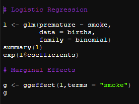
Another way to conduct this analysis is to do a logistic regression:
l <- glm(premature ~ smoke,
         data = births,
         family = binomial)
summary(l)
exp(l$coefficients)
When we look at the summary of l, we see that the coefficient (log odds ratio) of smoker is 0.2427 and that it’s p-value (the probability that chance had a say in the results) is 0.618:
Call:
glm(formula = premature ~ smoke, family = binomial, data = births)

Deviance Residuals:
    Min       1Q   Median       3Q      Max
-0.5905  -0.5905  -0.5278  -0.5278   2.0200

Coefficients:
            Estimate Std. Error z value Pr(>|z|)
(Intercept)  -1.9010     0.2973  -6.393 1.63e-10 ***
smokesmoker   0.2427     0.4871   0.498    0.618
---
Signif. codes:  0 ‘***’ 0.001 ‘**’ 0.01 ‘*’ 0.05 ‘.’ 0.1 ‘ ’ 1

(Dispersion parameter for binomial family taken to be 1)

    Null deviance: 121.49  on 149  degrees of freedom
Residual deviance: 121.24  on 148  degrees of freedom
AIC: 125.24

Number of Fisher Scoring iterations: 4
And, when we exponentiate the log odds ratio (0.2427), we come up with the same odds ratio from before:
> exp(l$coefficients)
(Intercept) smokesmoker
  0.1494253   1.2747253
Again, we’re saying that smokers have 27% higher odds than non-smokers. If you’re well-versed in statistics and epidemiology, this is enough to you. You understand what is going on. However, not everyone knows the dark arts. For them, I recommend giving the marginal effects.
In essence, marginal effects show your audience what the probability of the outcome is in both groups, the difference of that probability from one group to another, and — if it includes the confidence interval — whether or not those differences are significant (whether or not the observed differences have a good probability of being just by chance).
To do this, you could look at the exponentiated intercept above (13 / 87 = 0.1494253) and recognize it as the odds of premature birth if the mother was non-smoker. We could then use the Odds / 1+Odds = Probability formula to calculate the probability of premature births in non-smokers, which is 13%. (This makes sense, right? 13 of 100 mothers who did not smoke had premature babies.)
Next, the probability in smokers is the sum of the intercept (-1.9010) and the estimate/coefficient for smokers (0.2427), which is -1.6583. Exponentiate that log odds and you get 0.19. Convert that to probability by using the Odds / 1 + Odds formula, getting you 16%. So there is a 3% difference in probability between smokers and non-smokers.
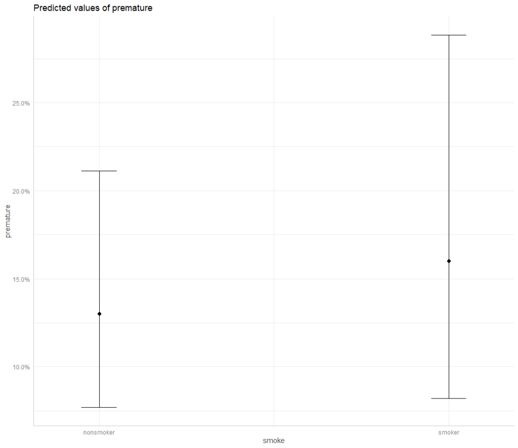
Now, here is a quick way to do this in R using the ggeffects package:
g <- ggeffect(l,terms = "smoke")
g
Which gives you:
# Predicted values of premature
# x = smoke

         x predicted std.error conf.low conf.high
 nonsmoker      0.13     0.297    0.077     0.211
    smoker      0.16     0.386    0.082     0.289
Now, you can see that the two have different probabilities, but that even the 95% confidence interval (conf.low to conf.high) overlaps. That overlap, just like with the odds ratio confidence interval, tells us that these differences in probabilities are not statistically significant.
You can even plot these predicted values and their confidence intervals:
r <- plot(g,
          facets = F,
          ci.style = "errorbar")
r
Which gives you:
A little bit of code can make that graph prettier with the ggplot package:
q <- r +
  geom_bar(stat = "identity",
           color = "blue",
           fill = "blue",
           alpha = 0.3) +
  theme_classic() +
  scale_y_continuous(labels = scales::percent_format(accuracy = 1)) +
  geom_label(aes(label = round(predicted,3)*100),
             nudge_y = -0.10,
             color = "black",
             size = 16) +
  labs(x = "Smoking Status",
       y = "Predicted Value of Premature Birth Proportion",
       title = "Proportion of Premature Births by Smoking Status in a Random Sample of 150 Births",
       subtitle = "Open Intro Data -- EXAMPLE") +
  theme(axis.text.x = element_text(size = 12, face = "bold" , color = "black", angle = 90),
        axis.text.y = element_text(size = 12, face = "bold", color = "black"),
        axis.title.x = element_text(size = 14, face = "bold", color = "black"),
        axis.title.y = element_text(size = 13, face = "bold", color = "black"),
        panel.grid.major.y = element_line(color = "red", linetype = "dashed", size = 0.1),
        plot.background = element_rect(fill = "transparent"))
q
The final plot looks a little like this:
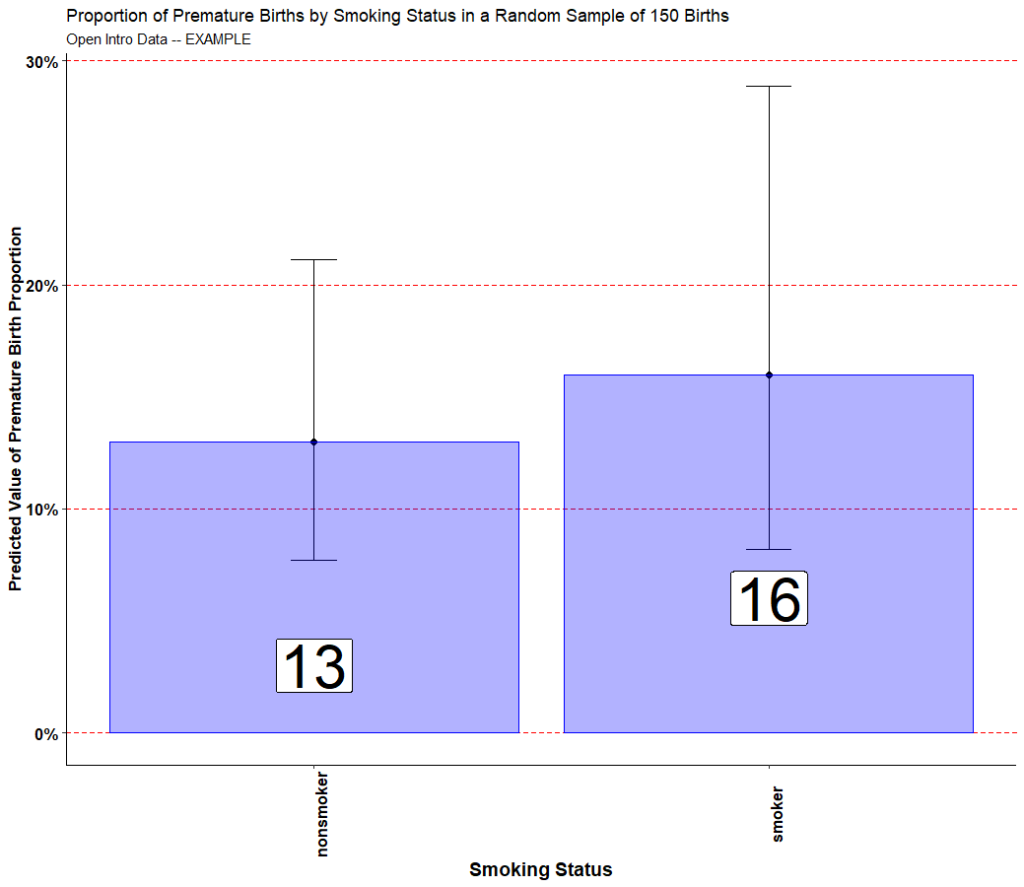
So, is there a difference in premature births between smokers and non-smokers in our sample? Yes, but the observed difference has a good probability of being just by chance.
Which one do you like better? A presentation of the odds ratio and respective 95% confidence interval, or a presentation of the marginal effects with its own confidence interval? On the one hand, the odds ratio tells you the difference in odds between the two groups, and whether or not that difference increases or decreases the odds of the outcome in the group being compared at baseline (non-smokers, in our example).
On the other hand, marginal effects can tell us about the reference group (non-smokers) and the groups we are comparing to that reference group (smokers). If you have a logistic regression with more terms, you would be able to see the predicted probability in the different groups after adjusting for the values in other groups. It’s all a matter of preference, really, and how you want to tell your story.

Chuckles, as I was examining some numbers and percentages over testicular cancer in law enforcement officers who used a rather old speed trap radar unit, infamously nestled close to their, ahem, family jewels.
Ran into one quality study, which suggested a 4% rate among all LEO’s (uncertain as to how the control group was chosen) and since, the technology was changed to trigger on, not always on, confounding things by a lot.
Germ cells are sensitive, especially when replicating and in males, that’s essentially incessantly, thermal input beyond what is acceptable and bodily mechanisms cannot relieve the excess thermal contribution might cause a problem.
Or someone tortured the data until it submitted, add moral scare.
Entirely unsure. It’s not like I’m about to bake my bowling balls in a microwave, then try to insert my fingers. 😉
And I’m not about to sign out the other form of balls from my wife’s locker, where she keeps me safe from unintentional self-harm. 😉
Trust me, that’s a mutual joke between us, all around.
As well as the shortsightedness of the Almighty, giving a man two heads, but only enough blood to operate one at a time.
LikeLike