Calculating TB Exposure Time Using R
Suppose that you have two cases of active tuberculosis (TB), and you want to determine the number of hours ten people were exposed to them. For this, you need to know the times that your TB cases were infectious in the location where your contacts, uh, contacted them.
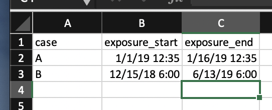
In this scenario, I have two cases: Case A was infectious from January 1, 2019, at 12:35 PM to January 31, 2019, at 9:30 AM. Case B was infectious from December 15, 2018, at 3:50 AM to March 14, 2019, at 10:50 AM. In real life, we don’t really know the exact time that someone became infectious. Heck, most of the time we use the average times we have in the literature to determine infectious periods, but just bare with me on this one.
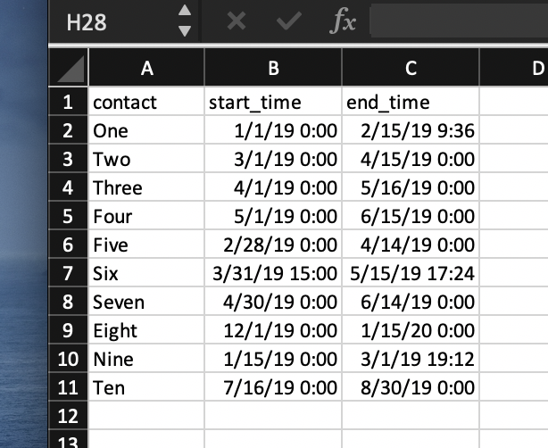
Now, suppose that we’ve done some interviews and found out that ten people (Contacts “One” through “Ten”) may have come into contact with our two infectious people. Under TB investigation guidelines:
“The likelihood of infection depends on the intensity, frequency, and duration of exposure. For example, airline passengers who are seated for >8 hours in the same or adjoining row as a person who is contagious are much more likely to be infected than other passengers. One set of criteria for estimating risk after exposure to a person with pulmonary TB without lung cavities includes a cut-off of 120 hours of exposure per month. However, for any specific setting, index patient, and contacts, the optimal cut-off duration is undetermined. Administratively determined durations derived from local experience are recommended, with frequent reassessments on the basis of results.”
You could just put it all on paper and determine the amount of time the contacts spent with the cases, but that would get out of control quickly if you start dealing with hundreds of contacts and dozens of cases. I tried doing this in Excel, but the number of IFTHEN statements that I had to write just got to be too much: “If the starting time for CASE ONE is between Date 1 and Date 2, then this and that…” It got to be too much.
So I decided to try it out in R. In very few lines of code, I was able to calculate the number of hours each contact spent with the cases.
First, the data… For this, I created an Excel workbook. On one spreadsheet, named “cases,” I put the cases. On another, named “contacts,” I put the contacts. Pretty self-explanatory, right. For each case, I logged the exposure time and end (infectious period). For each contact, I logged the contact times with the cases. In this scenario, case A and case B were in a building and spent time with the ten contacts at the times and dates that the ten contacts reported. Here’s what it looks like:
And…
Again, you could probably do this by hand by comparing case A and contact One, then A and Two and so forth. But let’s do it in R. First, the libraries:
library(tidyverse)
library(readxl)
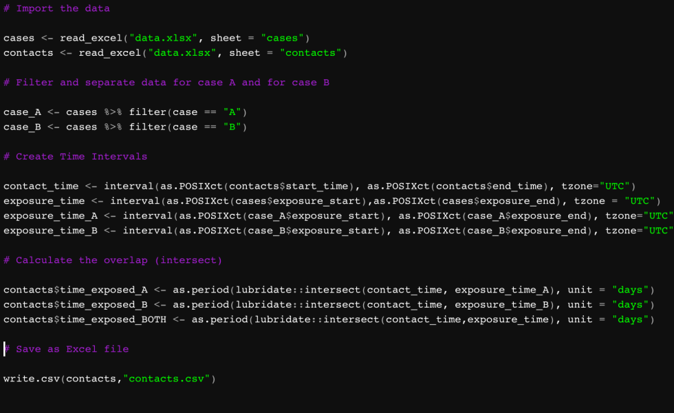
library(DescTools)Tidyverse will help us handle dates and data manipulation. Readxl will help read the Excel files. And DescTools will help with descriptive statistics. Next, we import the data:
cases <- read_excel("data.xlsx", sheet = "cases")
contacts <- read_excel("data.xlsx", sheet = "contacts")
Now, I’m interested in the exposure to each contact, instead of the overall contact to both cases. So I’m going to split up the contact times for each contact. (You can see where this can get tedious if done for each case when the case count is high. For that, I would create a loop.)
case_A <- cases %>% filter(case == "A")
case_B <- cases %>% filter(case == "B")
Now, I’m going to create time intervals. One for each contact, and the two for case A and case B.
contact_time <- interval(as.POSIXct(contacts$start_time), as.POSIXct(contacts$end_time), tzone="UTC")
exposure_time_A <- interval(as.POSIXct(case_A$exposure_start), as.POSIXct(case_A$exposure_end), tzone="UTC")
exposure_time_B <- interval(as.POSIXct(case_B$exposure_start), as.POSIXct(case_B$exposure_end), tzone="UTC")
Next, we need to know how many hours of overlap there are between each contact time and each exposure_time_A and exposure_time_B. The following code asks R to use lubridate (part of the tidyverse package) to calculate the intersection of each contact_time and the respective exposure times. From that calculation, we create the variables time_exposed_A and time_exposed_B that we will append to the contacts dataset.
contacts$time_exposed_A <- as.period(lubridate::intersect(contact_time, exposure_time_A), unit = "hours")
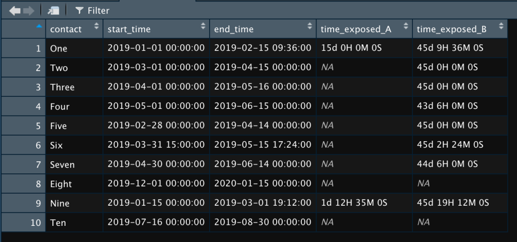
contacts$time_exposed_B <- as.period(lubridate::intersect(contact_time, exposure_time_B), unit = "hours")In the end, we can look at our data in contacts and see the number of hours each contact was exposed to each case, if they were exposed at all:
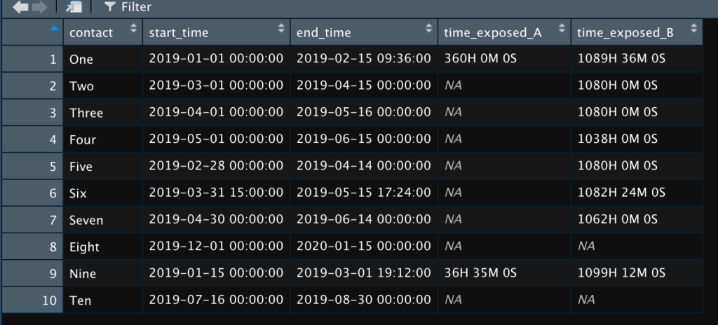
As you can see, contacts One and Nine were exposed to case A. All of the contacts except Eight and Ten were exposed to case B. If I wanted to know just the number of days, I’d go to the code above and change “hours” to “days” to get this:
And that’s it. Now you know exactly how much time each contact spent with each case. Simple, right? One more line of code and you can save this data in another spreadsheet that you can use for whatever it is you kids use spreadsheets for nowadays.
