Black Boxes and the Cochran-Mantel-Haenszel Equation

There’s this funny thing that happens in biostatistics where not being careful in how you collect and analyze your data may lead to this effect called confounding. Confounding happens when you see an association between X and Y, but it’s actually Z that is the real cause for Y. I often explain it with a quick example with coffee drinking.

In a study of pancreatic cancer, it is found that coffee drinkers have higher odds of pancreatic cancer than those who don’t drink coffee. However, if you account for the fact that smokers are also more likely to drink coffee, you find out that coffee drinkers who smoke are at highest risk, followed by smokers who don’t drink… Drinking coffee is not what’s causing the cancer. It’s the smoking.

To figure out the exact odds of cancer in coffee drinkers versus non-drinkers, and drinkers who smoke and drinkers who don’t smoke, etcetera, etcetera, we use the Cochran-Mantel-Haenszel equation. It answers the question: What are the odds of disease given the exposure, adjusting for all confounding variables?

Frankly, a logistic regression is easier — in my opinion — but this is how we learn biostatistics, by doing the tough math first. Anyway, I’m going to use some data from North Carolina to show you how the equation is done in R. Then I’ll do it by hand to show you that the R function works. Because that’s the gist of this blog post. You can’t just assume that the functions in R work.

Or you could just go on faith that they work and run the risk of being surprised. Yes, there are R packages that have mistakes in them, hence the need to be up to date on the latest version and to report any bugs you run into. Otherwise, you could be making a mistake in your conclusions if you use faulty conclusions from faulty software.

So do yourself a favor and do come math by hand just to make sure things are working right. If you don’t want to do it by hand, then at least take the time in your R script to write out some of the calculations to make sure.

Alright. In the words of the girl without fear, “Let’s do this!”

The Data

For this exercise, I’m going to use data from the OpenIntro package. I highly recommend this package if you want to play with R and some big datasets to hone your abilities. I’m also going to use the tidyverse, Hmisc, questionr and stats packages.

# Libraries
library(tidyverse)
library(openintro)
library(Hmisc)
library(questionr)
library(stats)

# Load data from OpenIntro

data(ncbirths)

d <- ncbirths[complete.cases(ncbirths), ]

# Look at the variables in the data

summary(d)

The Tables

Next, I’m going to make some tables to show the number of premature births from moms who smoke and moms who don’t smoke. The first table is for all moms. The second table is for white moms. The third table is for non-white moms.

# First table

t1 <- table(d$habit,d$premie)
t1

# Second table, white moms only

white <- d %>% filter(whitemom == "white")

t2 <- table(white$habit, white$premie)
t2

# Third table, non-white moms only

nonwhite <- d %>% filter(whitemom == "not white")

t3 <- table(nonwhite$habit, nonwhite$premie)
t3

The Odds Ratio

Traditionally, we’d calculate the odds ratio (the difference in odds of disease between the exposed and the unexposed groups) by splitting up the table into four cells and naming each cell A through D. The formula for the odds ratio is then to divide the product of A times D by the product of B times C. This tells us how much higher/lower odds the exposed group has compared to the unexposed group.

In R, just use the odds.ratio function from the questionr package:

# Odds ratio of each table

odds.ratio(t1) # Overall Odds Ratio
odds.ratio(t2) # Odds Ratio in White Moms
odds.ratio(t3) # Odds Ratio in non-White Moms

Here are the results of the code above:

> odds.ratio(t1) # Overall Odds Ratio
                   OR   2.5 % 97.5 %      p
Fisher's test 1.49223 0.75962 2.7742 0.2317
> odds.ratio(t2) # Odds Ratio in White Moms
                   OR   2.5 % 97.5 %      p
Fisher's test 1.72018 0.81759 3.4026 0.1221
> odds.ratio(t3) # Odds Ratio in non-White Moms
                    OR    2.5 % 97.5 % p
Fisher's test 0.916025 0.093719 4.5522 1

That’s 1.49, 1.72 and 0.92, respectively. This tells us that in all women, smoking women had about 49% higher odds of a premature baby if they smoked. In white women, the odds were 72% higher if they smoked. In non-White women, the odds were about 8% lower. Don’t pay too close attention to this as it is fake data. Nevertheless, the fact that it went from 72% higher to 8% lower between White and non-White women tells us that race might be a confounder here because the respective odds ratio of the two groups is different than the overall ratio.

So, to account for differences in race, let’s do the Cochran-Mantel-Haenszel equation.

The Cochran-Mantel-Haenszel Method for Doing Odds Ratio Good and Well

First, I did it the long way, by sticking to the formula given in the textbooks:

# Mantel-Haenszel... The Long Way

numerator <- ((13*484)/618) + ((2*141)/182)
denominator <- ((63*58)/618) + ((11*28)/182)

m_h <- numerator/denominator

My adjusted odds ratio was 1.54, meaning that women who smoked had 54% higher odds of a preemie baby compared to non-smokers, accounting for race. Now, let’s use the mantelhaen.test function from the stats package. First, I create an array of my values:

# Mantel-Haenszel... The quick way

m1 <- matrix(c(484,63,58,13), nrow = 2, byrow = T) # Matrix table of white moms
colnames(m1) <- c("FullTerm", "Preemie")
rownames(m1) <- c("NonSmoker", "Smoker")

m2 <- matrix(c(141,28,11,2), nrow = 2, byrow = T) # Matrix table of nonwhite moms
colnames(m2) <- c("FullTerm", "Preemie")
rownames(m2) <- c("NonSmoker", "Smoker")

array1 <- array(c(m1,m2), dim = c(2,2,2))

And then, the test:

mantelhaen.test(array1)

The result of that? Same result as what I got above, 1.54.

Illuminating the Black Box

Doing the work “the long way” allowed me to verify that the mantelhaen.test works the way it should. If it didn’t, I would have been shooting an email off to the developers to have them check out their function. Again, this is something you should always do at least once with new packages and new functions you’re using just to make sure they work the way they should.

Now, let’s do it all by hand…

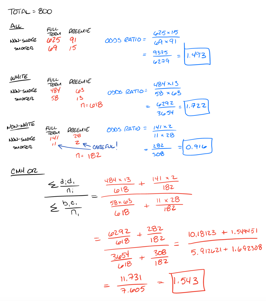
So, yeah, it checks out. The functions used to calculate the individual tables’ odds ratios work, and the function for the Cochrane-Mantel-Haenszel also seems to work well. As I noted in the hand-made calculations, be careful when your cell sizes get too small. In this case, there were only 2 non-white women who smoked and birthed premature children. Drawing conclusions on such a small number is a big no-no in epidemiology because it could be just by chance that this was the case.

In fact, the output for the mantelhaen.test function tells us that the association between smoking and premature birth weight, even when adjusting for race, is not significant. Just look at the 95% confidence interval:

Mantel-Haenszel chi-squared test with continuity correction

data:  array1
Mantel-Haenszel X-squared = 1.5539, df = 1, p-value = 0.2126
alternative hypothesis: true common odds ratio is not equal to 1
95 percent confidence interval:
 0.8445521 2.8172775
sample estimates:
common odds ratio 
          1.54251 

One Last Time

I cannot emphasize one more time how important it is that you verify that functions from packages you load are working the way they are intended. Those packages and functions are written by humans, so they’re prone to human errors. Black boxes of all kinds throughout history have led people astray, and some of the statistical/biostatistical work you do with R is much too important to let a bug in the programming mess it all up.

There are much more complicated functions and procedures in biostatistics that require quite a bit of time to do if you do them by hand. But, again, it’s worth doing once before the full analysis in order to make sure it’s all working the way it should. If you find yourself with some massive task, then do a key task by hand to make sure it’s all working well. And, as always, make sure to report those bugs you find so that the programmers can improve their product.