The Relationship Between Binge Drinking and COVID-19 Cases May Be Linear, But…

NOTE: This blog post has apparently been living rent-free in Dr. Glazer’s head for a couple of days. Instead of pointing out that his thesis may be incorrect, Dr. Glazer keeps pointing out that I mention that the data have to be normally distributed for the linear regression to work. In fact, the residuals from the linear regression need to be normally distributed for the statistical inference you gain from the linear regression (e.g. the p-value) to be correct. I apologize for this mistake/oversight/whatever.

The lesson is that no, binge drinking does not predict nor explain COVID-19 cases, but that is not what bothers Dr. Glazer, apparently. It’s the goddamned normality assumption that I mention.

Enjoy…

Look, I like economists. I really do. I follow their advice closely when it has to do to the economy and economic decisions that I make. However, a lot of them lately have been dabbling in epidemiology and biostatistics, and it makes me all sorts of itchy. It’s not that their statements are wrong, per se. It’s just that, sometimes, they say some things that are misleading… Or misled.

A few days ago, Amihai Glazer, PhD, tweeted out (and today corrected) the following message:

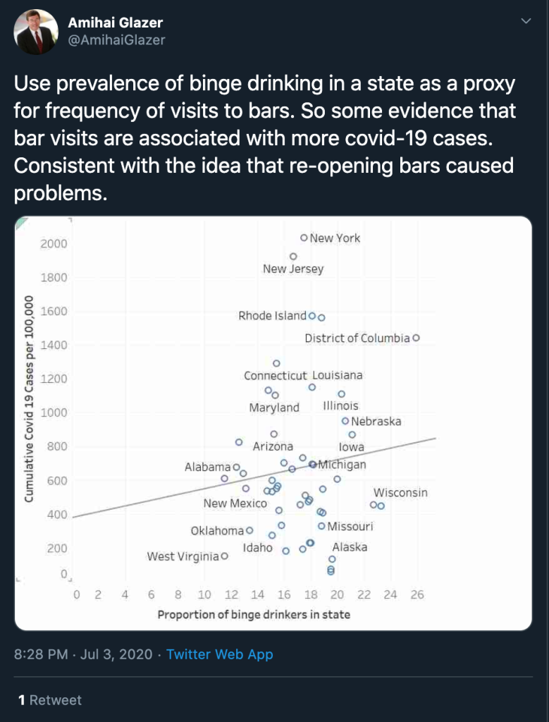
In epidemiology — like in many sciences — we start from a plausible idea and expand on it to prove our theories. In the tweet above, Dr. Glazer, uses a linear regression to show that there is an association between the proportion of binge drinkers in a state and the cumulative cases of COVID-19. This led to many criticisms, many pointing out that a simple linear regression is not enough to reach this conclusion.

Those criticizing this approach are correct. While the line of best fit does point up and to the right, it doesn’t mean that the more binge drinkers a state has, the more likely it is that it will have COVID-19 cases. In other words, if I tell you the proportion of binge drinkers a state has, you cannot predict the number (or rate per 100,000) of COVID-19 cases that state has.

In epidemiology and biostatistics, we try hard to make sure that these models are predictive in that sense. We look at all the factors that would go into such an association. For example, Dr. Glazer is right in that crowded bars are a source of contagion, so it stands to reason that more drinking equals more cases. But that is a very simplistic way of looking at it. There are a lot of factors that go into this, like differences in gender of drinkers, the drinking habits (at home or at the bar) of binge drinkers, and so on and so forth.

When it comes to linear regression — which is what Dr. Glazer seems to have tried here — there are some rules your data must follow (or you must follow in setting up your data) to make sure the model works the way it should. One of those rules is that your data needs to be normally distributed. (This is part of the Central Limit Theorem, which allows for statistical inference, but that is a whole lecture I don’t have time to give you.) So let’s take a quick look at the distribution of the percentage of binge drinkers in the 50 states:

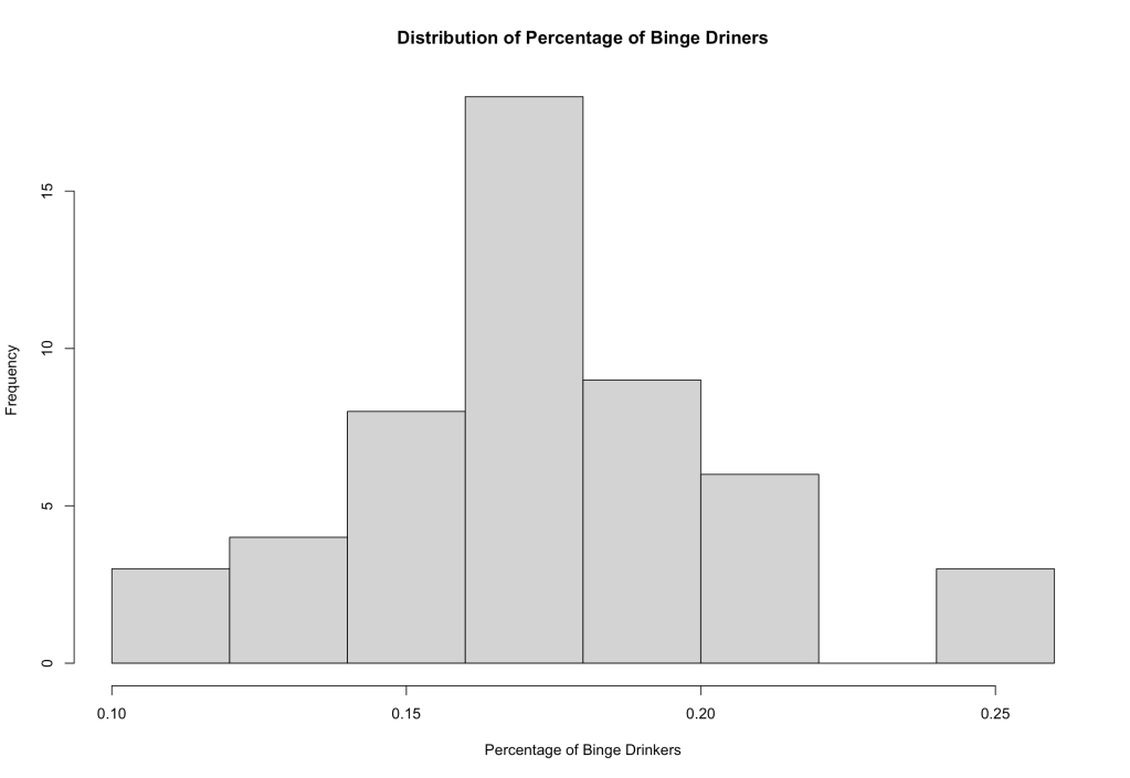
Okay, so the percentage of binge drinkers is more or less normally distributed. We’re good here. What about the rate per 100,000 of COVID-19 cases? Well:

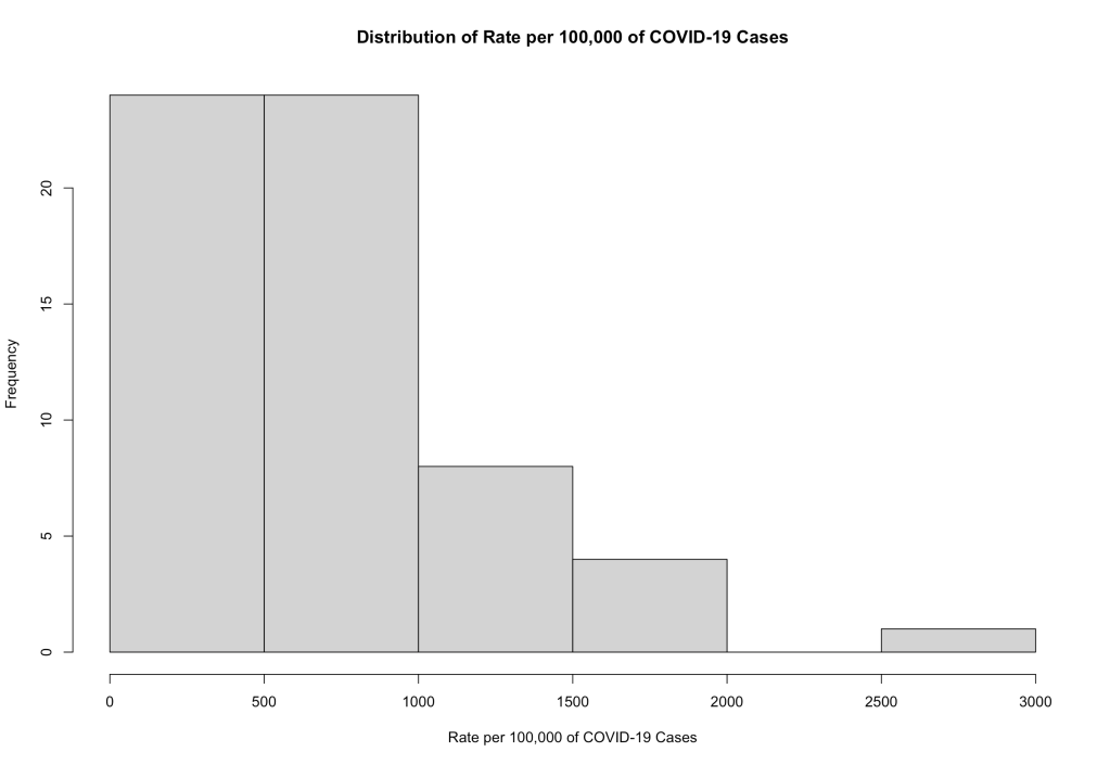
The assumptions of a linear regression fall apart here if we were to look at the rate of 100,000 as a predicted measure from the predictor (percentage binge drinking). To fix this, we can “transform” the data to make it normal. (When we are interpreting the results, we need to make sure to transform back to the original form, though. A rookie mistake I’ve made many times.)

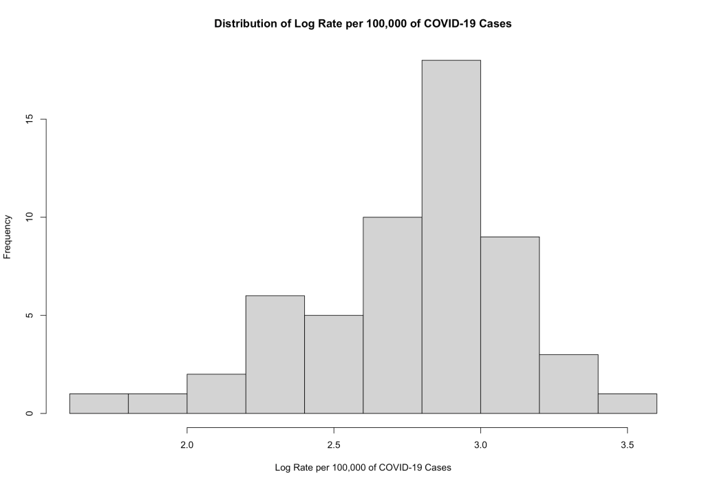
So it’s a little skewed, but it is definitely more normal. What if you can’t transform your data? Well, then you use other statistical methods. Again, that’s a whole lecture — or even a series of lectures. So lucky for us that these data transformed alright. However, from the looks of things, Dr. Glazer didn’t do this. To the uninitiated, his graph and the line tell a story… But it’s a story whose conclusions are flawed because of the simple fact that the rates per 100,000 are not normally distributed.

We can still do a regression, but the amount of the variance in the rates that is explained by the percentage of binge drinkers (what some call the r-squared) is not a lot. Let me show you with some processing in R.

glm(formula = rate ~ Percentage, data = d)
Deviance Residuals: 
    Min       1Q   Median       3Q      Max  
-634.60  -285.31   -59.48   165.56  1208.82  
Coefficients:
            Estimate Std. Error t value Pr(>|t|)  
(Intercept)    908.5      354.4   2.564   0.0135 *
Percentage   -1074.3     2033.3  -0.528   0.5997  
---
Signif. codes:  0 ‘***’ 0.001 ‘**’ 0.01 ‘*’ 0.05 ‘.’ 0.1 ‘ ’ 1
(Dispersion parameter for gaussian family taken to be 183990.4)
    Null deviance: 8882900  on 49  degrees of freedom
Residual deviance: 8831537  on 48  degrees of freedom
AIC: 751.98
Number of Fisher Scoring iterations: 2

This linear regression tells us that there is no statistically significant association between the rate and the percentage of binge drinkers (p = 0.5997). Not only that but the coefficient of determination (the proportion of the variation in rates that is explained by the binge drinking proportions) is 0.005782202. This means that 0.06% of the variation in rates is explained by the percentage.

Visually, it looks like this:

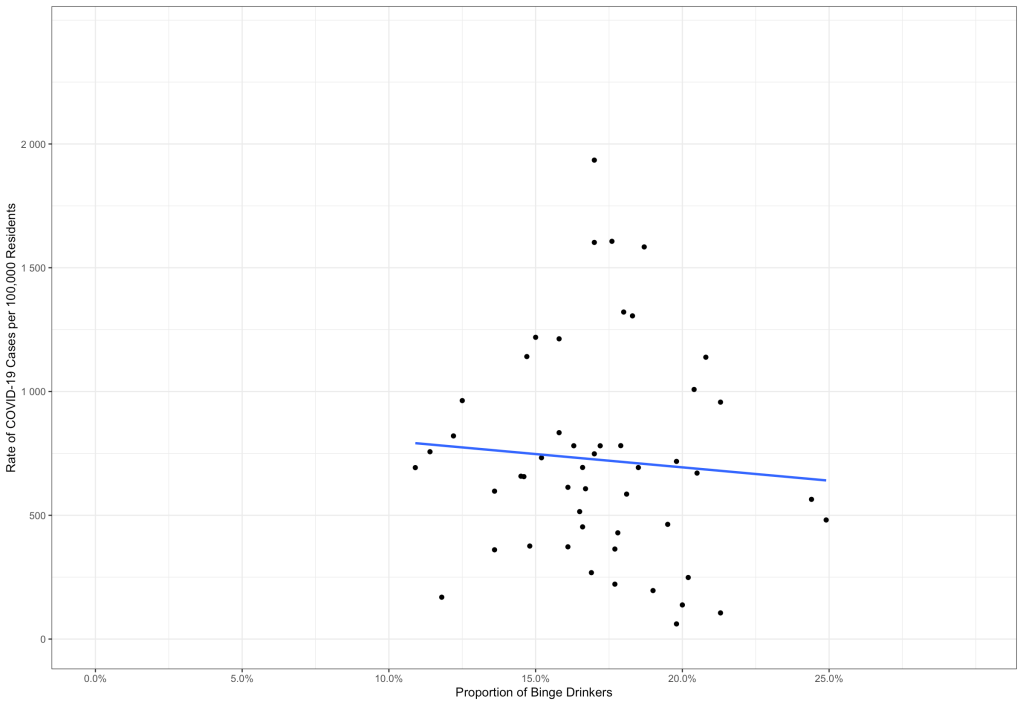
It doesn’t look at all like what Dr. Glazer put out there, thought the data sources are both CDC. Oh, well… Remember that we need to get the log of the rate for the linear regression to be valid. The results above are not valid. So let’s do it with the log of the rate per 100,000.

Call:
glm(formula = rate.log ~ Percentage, data = d)
Deviance Residuals: 
     Min        1Q    Median        3Q       Max  
-0.94007  -0.12563   0.05016   0.13752   0.51429  
Coefficients:
            Estimate Std. Error t value Pr(>|t|)    
(Intercept)   3.0486     0.2589  11.774 9.28e-16 ***
Percentage   -1.6249     1.4856  -1.094     0.28    
---
Signif. codes:  0 ‘***’ 0.001 ‘**’ 0.01 ‘*’ 0.05 ‘.’ 0.1 ‘ ’ 1
(Dispersion parameter for gaussian family taken to be 0.09821905)
    Null deviance: 4.8320  on 49  degrees of freedom
Residual deviance: 4.7145  on 48  degrees of freedom
AIC: 29.825
Number of Fisher Scoring iterations: 2

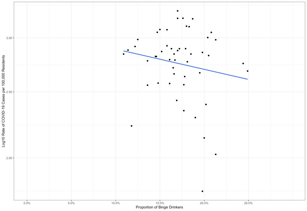
In this model, the AIC (a measure of how good the model fits) is much lower than the first model because the data are normal. And the r-squared? Here, it is 0.02431699. This means that about 2% of the variation in the log of the rate is explained by the percentage of binge drinkers, which itself is not statistically significant (p = 0.28). In other words, there is a good chance that the line we see in the scatter plot is actually flat in the population, and we just see it sloped because of the sample we took. Here’s that scatter plot:

So What Have We Learned?

First, Dr. Glazer should have known better than to put this on Twitter just like that, in my opinion. People with his academic pedigree (a PhD from Yale) have a sort of authority in these matters, and him putting it out like that may make people come to the wrong conclusion. Second, without the proper foundation in statistics, the conclusion is full-on wrong. Third, even when the data are properly set up for the linear regression, the association is super-weak, and not even statistically significant. The line has a good chance of being flat in the population based on the sample we’re looking at.

Personally, I’ve learned that I need to have all my ducks in a row before going public with any findings from my self-directed data analyses. So please be responsible and remember L.I.N.E. when it comes to linear regression… Your data must be Linear, Independent, Normal and with Equal Variances.